Johnny Deng's Column: Sinc Function, Rect Function

Rectangular Function

Rectangular function

The rectangular function (also known as the rectangle function, rect function, unit pulse, or the normalized boxcar function) is defined as,

$\text{[math]}$

$\text{[math]}$ \frac{1}{2} \\[3pt] \frac{1}{2} & \mbox{if } |t| = \frac{1}{2} \\[3pt] 1 & \mbox{if } |t| < \frac{1}{2} \end{cases} " src="http://upload.wikimedia.org/math/0/2/d/02dfb78ddb6c1f88b062ca0d076ef26f.png">

Alternate definitions of the function define $\mathrm{rect}(\pm \begin{matrix} \frac{1}{2} \end{matrix})$ to be 0, 1, or undefined. We can also express the rectangular function in terms of the Heaviside step function, $u (t)$ :

$\mathrm{rect}\left(\frac{t}{\tau}\right) = u \left( t + \frac{\tau}{2} \right) - u \left( t - \frac{\tau}{2} \right)$

or, alternatively:

$\mathrm{rect}(t) = u \left( t + \frac{1}{2} \right) \cdot u \left( \frac{1}{2} - t \right)$

The rectangular function is normalized:

$\int_{-\infty}^\infty \mathrm{rect}(t)\,dt=1$

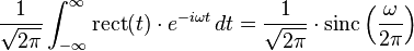
The unitary Fourier transforms of the rectangular function are,

$\frac{1}{\sqrt{2\pi}}\int_{-\infty}^\infty \mathrm{rect}(t)\cdot e^{-i \omega t} \, dt =\frac{1}{\sqrt{2\pi}}\cdot \mathrm{sinc}\left(\frac{\omega}{2\pi}\right)$ ,

and, in terms of the normalized sinc function,

$\int_{-\infty}^\infty \mathrm{rect}(t)\cdot e^{-i 2\pi f t} \, dt = \mathrm{sinc}(f)$

We can define the triangular function as the convolution of two rectangular functions:

tri(t) = rect(t) * rect(t)

Viewing the rectangular function as a probability distribution function, its characteristic function is,

$\varphi(k) = \frac{\sin(k/2)}{k/2}\,$

and its moment generating function is,

$M(k)=\frac{\mathrm{sinh}(k/2)}{k/2}\,$

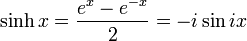
where $sinh(t)$ is the hyperbolic sine function.

Hyperbolic function

A ray through the origin intercepts the hyperbola

x 2 - y 2 = 1

in the point

(cosh a,sinh a)

, where

a

is the area between the ray, its mirror image with respect to the

x

-axis, and the hyperbola (see animated version with comparison with the trigonometric (circular) functions).

In mathematics, the hyperbolic functions are analogs of the ordinary trigonometric, or circular, functions. The basic hyperbolic functions are the hyperbolic sine "sinh", and the hyperbolic cosine "cosh", from which are derived the hyperbolic tangent "tanh", etc., in analogy to the derived trigonometric functions. The inverse functions are the inverse hyperbolic sine "arsinh" (also called "arсsinh" or "asinh") and so on.

Just as the points (cos t, sin t) define a circle, the points (cosh t, sinh t) define the right half of the equilateral hyperbola. Hyperbolic functions are also useful because they occur in the solutions of some important linear differential equations, notably that defining the shape of a hanging cable, the catenary, and Laplace's equation (in Cartesian coordinates), which is important in many areas of physics including electromagnetic theory, heat transfer, fluid dynamics, and special relativity.

The hyperbolic functions take real values for real argument called a hyperbolic angle. In complex analysis, they are simply rational functions of exponentials, and so are meromorphic.

Standard algebraic expressions

sinh, cosh and tanh

csch, sech and coth

The hyperbolic functions are:

Hyperbolic sine, often pronounced "shine" or "sinch":

$\sinh x = \frac{e^x - e^{-x}}{2} = -i \sin ix \!$

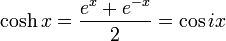
Hyperbolic cosine, often pronounced "cosh" or "co-shine":

$\cosh x = \frac{e^{x} + e^{-x}}{2} = \cos ix \!$

Hyperbolic tangent, often pronounced "than" or "tanch":

$\tanh x = \frac{\sinh x}{\cosh x} = \frac {e^x - e^{-x}} {e^x + e^{-x}} = \frac{e^{2x} - 1} {e^{2x} + 1} = -i \tan ix \!$

Hyperbolic cotangent, often pronounced "coth" or "chot":

$\coth x = \frac{\cosh x}{\sinh x} = \frac {e^x + e^{-x}} {e^x - e^{-x}} = \frac{e^{2x} + 1} {e^{2x} - 1} = i \cot ix \!$

Hyperbolic secant, often pronounced "sheck" or "sech":

$\operatorname{sech} x = \frac{1}{\cosh x} = \frac {2} {e^x + e^{-x}} = \sec {ix} \!$

Hyperbolic cosecant, often pronounced "cosheck" or "cosech"

$\operatorname{csch} x = \frac{1}{\sinh x} = \frac {2} {e^x - e^{-x}} = i\,\csc\,ix \!$

where $i$ is the imaginary unit.

The complex forms in the definitions above derive from Euler's formula.

Useful relations

$\sinh(-x) = -\sinh x\,\!$

$\cosh(-x) = \cosh x\,\!$

Hence:

$\tanh(-x) = -\tanh x\,\!$

$\coth(-x) = -\coth x\,\!$

$\operatorname{sech}(-x) = \operatorname{sech}\, x\,\!$

$\operatorname{csch}(-x) = -\operatorname{csch}\, x\,\!$

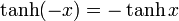
It can be seen that both cosh x and sech x are even functions, others are odd functions.

Standard Integrals

For a full list of integrals of hyperbolic functions, see list of integrals of hyperbolic functions

$\int\sinh cx\,dx = \frac{1}{c}\cosh cx + C$

$\int\cosh cx\,dx = \frac{1}{c}\sinh cx + C$

$\int \tanh cx\,dx = \frac{1}{c}\ln|\cosh cx| + C$

$\int \coth cx\,dx = \frac{1}{c}\ln|\sinh cx| + C$

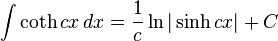
In the above expressions, C is called the constant of integration.

Taylor series expressions

It is possible to express the above functions as Taylor series:

$\sinh x = x + \frac {x^3} {3!} + \frac {x^5} {5!} + \frac {x^7} {7!} +\cdots = \sum_{n=0}^\infty \frac{x^{2n+1}}{(2n+1)!}$

$\cosh x = 1 + \frac {x^2} {2!} + \frac {x^4} {4!} + \frac {x^6} {6!} + \cdots = \sum_{n=0}^\infty \frac{x^{2n}}{(2n)!}$

$\tanh x = x - \frac {x^3} {3} + \frac {2x^5} {15} - \frac {17x^7} {315} + \cdots = \sum_{n=1}^\infty \frac{2^{2n}(2^{2n}-1)B_{2n} x^{2n-1}}{(2n)!}, \left |x \right | < \frac {\pi} {2}$

$\coth x = \frac {1} {x} + \frac {x} {3} - \frac {x^3} {45} + \frac {2x^5} {945} + \cdots = \frac {1} {x} + \sum_{n=1}^\infty \frac{2^{2n} B_{2n} x^{2n-1}} {(2n)!}, 0 < \left |x \right | < \pi$ (Laurent series)

$\operatorname {sech}\, x = 1 - \frac {x^2} {2} + \frac {5x^4} {24} - \frac {61x^6} {720} + \cdots = \sum_{n=0}^\infty \frac{E_{2 n} x^{2n}}{(2n)!} , \left |x \right | < \frac {\pi} {2}$

$\operatorname {csch}\, x = \frac {1} {x} - \frac {x} {6} +\frac {7x^3} {360} -\frac {31x^5} {15120} + \cdots = \frac {1} {x} + \sum_{n=1}^\infty \frac{ 2 (1-2^{2n-1}) B_{2n} x^{2n-1}}{(2n)!} , 0 < \left |x \right | < \pi$ (Laurent series)

where

$B_n \,$ is the nth Bernoulli number

$E_n \,$ is the nth Euler number

Sinc function

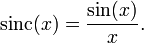
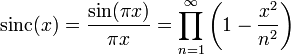
In mathematics, the sinc function, denoted by $\mathrm{sinc}(x)\,$ , has two definitions, sometimes distinguished as the normalized sinc function and unnormalized sinc function:

In digital signal processing and information theory, the normalized sinc function is commonly defined by
$\mathrm{sinc}(x) = \frac{\sin(\pi x)}{\pi x}.$
In mathematics, the historical unnormalized sinc function (for sinus cardinalis), is defined by
$\mathrm{sinc}(x) = \frac{\sin(x)}{x}.$

In both cases, the value of the function at the removable singularity at zero is sometimes specified explicitly as the limit value 1. The sinc function is analytic everywhere.

The term "sinc" is a contraction of the function's full name, the sine cardinal.

Properties

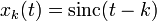
The normalized sinc(x) (blue) and unnormalized sinc function (red) shown on the same scale from x = −6π to 6π.

The normalized sinc function has properties that make it ideal in relationship to interpolation and bandlimited functions:

$\mathrm{sinc}(0) = 1\,$ and $\mathrm{sinc}(k) = 0\,$ for $k\ne 0\,$ and $k\in\mathbb{Z}\,$ (integers); that is, it is an interpolating function.
the functions $x_k(t)=\mathrm{sinc}(t-k) \$ form an orthonormal basis for bandlimited functions in the function space $L^2(\R)$ , with highest angular frequency $\omega_\mathrm{H}=\pi\,$ (that is, highest cycle frequency $f_\mathrm{H}=1/2\,$ ).

Other properties of the two sinc functions include:

The local maxima and minima of the unnormalized sinc, $\begin{matrix}\frac{\sin(x)}{x} \end{matrix}\,$ correspond to its intersections with the cosine function. That is, $\begin{matrix}\frac{\sin(x)}{x} \end{matrix} = \cos(x) \,$ for all points x where the derivative of $\begin{matrix}\frac{\sin(x)}{x} \end{matrix}\,$ is zero (and thus a local extremum is reached).

The unnormalized sinc is the zero^th order spherical Bessel function of the first kind, $j_0(x) = \begin{matrix}\frac{\sin(x)}{x} \end{matrix}\,$ . The normalized sinc is $j_0(\pi x)\,$ .

The zero-crossings of the unnormalized sinc are at nonzero multiples of $\pi\,$ ; zero-crossing of the normalized sinc 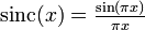$\mathrm{sinc}(x) = \begin{matrix}\frac{\sin(\pi x)}{\pi x} \end{matrix}\,$ occur at nonzero integer values.

The continuous Fourier transform of the normalized sinc $\mathrm{sinc}(x) = \begin{matrix}\frac{\sin(\pi x)}{\pi x} \end{matrix}\,$ (to ordinary frequency) is $\mathrm{rect}(f)\,$ .

$\int_{-\infty}^\infty \mathrm{sinc}(t)\,e^{-2\pi i f t}dt = \mathrm{rect}(f)$ ,

where the rectangular function is 1 for argument between –1/2 and 1/2, and zero otherwise.

The Fourier integral above, including the special case

$\int_{-\infty}^\infty \begin{matrix}\frac{\sin(\pi x)}{\pi x} \end{matrix}\, dx = \mathrm{rect}(0) = 1$

is an improper integral. It is not a Lebesgue integral because:

$\int_{-\infty}^\infty \left|\begin{matrix}\frac{\sin(\pi x)}{\pi x} \end{matrix}\right|\ dx = \infty \,$

$\mathrm{sinc}(x) = \frac{\sin(\pi x)}{\pi x} = \prod_{n=1}^\infty \left(1 - \frac{x^2}{n^2}\right)$

$\mathrm{sinc}(x) = \frac{\sin(\pi x)}{\pi x} = \frac{1}{\Gamma(1+x)\Gamma(1-x)}$

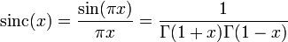
where

Γ(x)

is the gamma function.

$\int_{0}^{x} \frac{\sin(\theta)}{\theta}\,d\theta = Si(x)$

where Si(x) is the sine integral.

Relationship to the Dirac delta distribution

The normalized sinc function can be used as a nascent delta function, even though it is not a distribution.

The normalized sinc function is related to the delta distribution δ(x) by

$\lim_{a\rightarrow 0}\frac{1}{a}\textrm{sinc}(x/a)=\delta(x).$

This is not an ordinary limit, since the left side does not converge. Rather, it means that

$\lim_{a\rightarrow 0}\int_{-\infty}^\infty \frac{1}{a}\textrm{sinc}(x/a)\varphi(x)\,dx =\int_{-\infty}^\infty\delta(x)\varphi(x)\,dx = \varphi(0),$

for any smooth function $\varphi(x)$ with compact support.

In the above expression, as a approaches zero, the number of oscillations per unit length of the sinc function approaches infinity. Nevertheless, the expression always oscillates inside an envelope of ±1/(πx), regardless of the value of a. This contradicts the informal picture of δ(x) as being zero for all x except at the point x=0 and illustrates the problem of thinking of the delta function as a function rather than as a distribution. A similar situation is found in the Gibbs phenomenon.

Johnny Deng's Column

Thursday 2 August 2007

Sinc Function, Rect Function

Standard algebraic expressions

Useful relations

Standard Integrals

Taylor series expressions

Relationship to the Dirac delta distribution

No comments:

Site Search

Blog Archive

Who am I?

Access History