Hi all, This Blog is an English archive of my PhD experience in Imperial College London, mainly logging my research and working process, as well as some visual records.

Monday 3 September 2007

Linear regression

In statistics, linear regression is a regression method that models the relationship between a dependent variable Y, independent variables Xi, i = 1, ..., p, and a random term ε. The model can be written as

Example of linear regression with one dependent and one independent variable.

Example of linear regression with one dependent and one independent variable.
Y = \beta_1  + \beta_2 X_2 +  \cdots +\beta_p X_p + \varepsilon

where β1 is the intercept ("constant" term), the βis are the respective parameters of independent variables, and p is the number of parameters to be estimated in the linear regression. Linear regression can be contrasted with nonlinear regression.

This method is called "linear" because the relation of the response (the dependent variable Y) to the independent variables is assumed to be a linear function of the parameters. It is often erroneously thought that the reason the technique is called "linear regression" is that the graph of Y = β0 + βx is a straight line or that Y is a linear function of the X variables. But if the model is (for example)

Y = \alpha + \beta x + \gamma x^2 + \varepsilon

the problem is still one of linear regression, that is, linear in x and x2 respectively, even though the graph on x by itself is not a straight


Sample data.

Say we have a set of data, , shown at the left. If we have reason to believe that there exists a linear relationship between the variables x and y, we can plot the data and draw a "best-fit" straight line through the data. Of course, this relationship is governed by the familiar equation . We can then find the slope, m, and y-intercept, b, for the data, which are shown in the figure below.

Let's enter the above data into an Excel spread sheet, plot the data, create a trendline and display its slope, y-intercept and R-squared value. Recall that the R-squared value is the square of the correlation coefficient. (Most statistical texts show the correlation coefficient as "r", but Excel shows the coefficient as "R". Whether you write is as r or R, the correlation coefficient gives us a measure of the reliability of the linear relationship between the x and y values. (Values close to 1 indicate excellent linear reliability.))

Enter your data as we did in columns B and C. The reason for this is strictly cosmetic as you will soon see.


Linear regression equations.

If we expect a set of data to have a linear correlation, it is not necessary for us to plot the data in order to determine the constants m (slope) and b (y-intercept) of the equation . Instead, we can apply a statistical treatment known as linear regression to the data and determine these constants.

Given a set of data with n data points, the slope, y-intercept and correlation coefficient, r, can be determined using the following:


(Note that the limits of the summation, which are i to n, and the summation indices on x and y have been omitted.)


Implicitly applying regression to the sample data.

It may appear that the above equations are quite complicated, however upon inspection, we see that their components are nothing more than simple algebraic manipulations of the raw data. We can expand our spread sheet to include these components.

  1. First, add three columns that will be used to determine the quantities xy, x2 and y2, for each data point.

  2. Next, use Excel to evaluate the following: Sx, Sy, S(xy), S(x2), S(y2), (Sx)2, (Sy)2. Recall that the symbol, S, means "summation". Additionally, the term xy is the product of x and y, that is: x * y. Also, the term S(x2) is very different than the term (Sx)2. Be careful with your order of operations!

  3. Now use Excel to count the number of data points, n. (To do this, use the Excel COUNT() function. The syntax for COUNT() in this example is: =COUNT(B3:B8) and is shown in the formula bar in the screen shot below.

  4. Finally, use the above components and the linear regression equations given in the previous section to calculate the slope (m), y-intercept (b) and correlation coefficient (r) of the data. If you are careful, your spread sheet should look like ours. Note that our equations for the slope, y-intercept and correlation coefficient are highlighted in yellow.

Linear function

In mathematics, the term linear function can refer to either of two different but related concepts.

Usage in elementary mathematics

In elementary algebra and analytic geometry, the term linear function is often used to mean a first degree polynomial function of one variable. These functions are called "linear" because they are precisely the functions whose graph in the Cartesian coordinate plane is a straight line.

Such a function can be written as

f(x) = mx + b,

where m and b are real constants and x is a real variable. The constant m is often called the slope while b is the y-intercept, which gives the point of intersection between the graph of the function and the y-axis. Changing m makes the line steeper or shallower, while changing b moves the line up or down.

Three geometric linear functions — the red and blue ones have same slope (m), while red and green ones have same y-intercept (b).

Three geometric linear functions — the red and blue ones have same slope (m), while red and green ones have same y-intercept (b).

Examples of functions whose graph is a line include the following:

  • f1(x) = 2x + 1
  • f2(x) = x / 2 + 1
  • f3(x) = x / 2 − 1

The graphs of these are shown in the image at right.

Usage in advanced mathematics

In advanced mathematics, a linear function often means a function that is a linear map, that is, a map between two vector spaces that preserves vector addition and scalar multiplication.

A function f(x) = mx + b is a linear map if and only if b = 0. For other values of b this falls in the more general class of affine maps.

Spearman Correlation - Example

Example of Statistical Test using the Spearman Rank-Difference Correlation Coefficient

Is there a significant positive correlation between the rankings of 10 children on a reading test and their teacher's ranking of their reading ability? In this problem we are relating a set of scores (interval level of measurement) with the teacher's ranking of the children in reading (ordinal level of measurement). To do this we first convert the reading test scores to ranks by assigning the highest score a rank of 1, the next highest a rank of 2, etc. Now we are looking at rankings on two variables and can use the Spearman Rank-Difference Correlation Coefficient to test the significance of the relationship. The two set of ranks, as well as the difference between the pairs of ranks (D) and the differences squared (D2), are shown in the following table.

Worksheet to Calculate the Correlation between Students Ranks on a Reading Test and Teacher's Ranking of the Students on Reading
Reading Test
Score Rank
Teacher's Ranking
on Reading
D D2
1 3 -2 4
2 2 0 0
3 1 2 4
4 4 0 0
5 5 0 0
6 6 0 0
7 8 -1 1
8 7 1 1
9 10 -1 1
10 9 1 1
Total

12

From the table we can see that:

df = N - 2 = 10 - 2 = 8

We now have the information we need to complete the six step process for testing statistical hypotheses for our research problem.

  1. State the null hypothesis and the alternative hypothesis based on your research question.

    H0: rS = 0

    H1: rS > 0

    Note: Our null hypothesis states that there is no significant relationship between the two variables. The alternative hypothesis states that there is a significant positive correlation between the two variables.

  2. Set the alpha level.

    Note: As usual we will set our alpha level at .05, we have 5 chances in 100 of making a type I error.
  3. Calculate the value of the appropriate statistic. Also indicate the degrees of freedom for the statistical test if necessary.

    rS = .93

    df = N - 2 = 10 - 2 = 8

  4. Write the decision rule for rejecting the null hypothesis.

    Reject H0 if rS >= .549

    Note: To write the decision rule we had to know the critical value for rS, with an alpha level of .05, and 8 degrees of freedom. We can do this by looking at Appendix Table B, this is the same table we used for the Pearson r, and noting the tabled value for the column for the .10 level and the row for 8 df (.549).

    Note: We used the .10 column because we are doing a one-tailed test with an alpha of .05 As noted in our problem above the the Pearson r, in the table of critical values for r, the .10 column is used for alpha = .10 (two-tailed test) and for alpha = .05 (one-tailed test).

  5. Write a summary statement based on the decision.
    Reject H0, p < .05, one-tailed
    Note: Since our calculated value of rS (.93) is greater than .549, we reject the null hypothesis and accept the alternative hypothesis.
  6. Write a statement of results in standard English.
    There is a significant positive correlation between the children's ranks on a reading test and their teacher's ranking of them on reading.

Choosing the Proper Statistical Test


Let's finish our discussion of inferential statistics with a summary of all the inferential statistics we have discussed and look at the conditions under which we would use each of these statistics. Generally if we know the number of groups or samples in our research design and the level of measurement of the dependent variable we will know which inferential statistic to use.

First let us look at statistical hypotheses in research designs where the dependent variable is at the interval or ratio level. These statistics are known as parametric statistics and we have used the following:

  • If we are testing a statistical hypothesis, involving a single score (we are comparing the score with the population mean) we will use the z-score test (see lesson 9).
  • If we are testing a statistical hypothesis involving a single group (we are comparing the mean of the group with the population mean) and the standard deviation of the population is know use the z test (see lesson 10).
  • If we are testing a statistical hypothesis involving a single group (we are comparing the mean of the group with the population mean) and the standard deviation of the population is not known use the single sample t-test (see lesson 10).
  • If we are testing a statistical hypothesis involved two groups of subjects (we are comparing the means of the two groups) and the two groups are independent of one another, we use the independent t-test (see lesson 11).
  • If we are testing a statistical hypothesis involved two groups of subjects (we are comparing the means of the two groups) and the two groups are dependent on one another (pretest/posttest or matched samples), we use the dependent t-test (see lesson 12).
  • If we are testing a statistical hypothesis involved three or more groups of subjects (we are comparing the means of three or more groups) and there is a single dependent variable in the study, we use one-way analysis of variance (see lesson 13).
  • If we are testing a statistical hypothesis involved the relationship between two variables for one sample (we are measuring the relationship between the two variables) and the data is at the interval or ratio level of measurement), use the Pearson product moment correlation coefficient.

We also looked at two other statistics we could use with data that was not at the interval or ratio level of measurement. These statistics are called non-parametric statistics.

  • If we are testing a statistical hypothesis for one, two, or more groups with one or two variables where the data is catagorical (frequencies). The data is at the nominal level of measurement. For this type of study use chi-square (see lesson 14). We have discussed three different variants of the chi-square statistic.
    1. one variable chi-square with equal expected frequencies
    2. one variable chi-square with unequal (predetermined) expected frequencies
    3. two variable chi-square
  • If we are testing a statistical hypothesis involved the relationship between two variables for one sample (we are measuring the relationship between the two variables) and the data is at the ordinal level of measurement (ranks), use the Spearman rank-difference correlation coefficient (see lesson 15).

The information we have discussed above can be put into the following table. The table also includes other statistics that we have not included in this course. If you think you may need one of the statistics we did not cover in your research design, please send e-mail to the instructor and I will give you a reference to the calculation and interpretation of that statistic. I wish you the best as you complete the final examination for this course and as you apply the information from this course to your own research design.

Selecting a Statistical Test
Level of
Measurement
Sample Characteristics
One-Sample
Statistical
Tests
Two-Sample
Statistical
Tests
Multiple Sample
Statistical
Tests
Measures of
Association
(one-sample, more
than one variable)
Independent
Samples
Non-independent
Samples
Nominal or
Categorical
(frequencies)
Chi-Square Chi-Square McNemar
Change Test
Chi-Square Phi Coefficient
Ordinal
(Ranks)
Kolmagorov-Smirnov
One-Sample
Test
Mann Whitney
U-Test
Wilcoxon
Matched Pairs
Signed-Rank
Test
Krushcal-Wallis
One-Way
Analysis of
Variance
Spearman rho
rS
Interval
or Ratio
Z test

One-Sample
t-Test
Independent
t-test
Dependent
t-test
Simple
Analysis of Variance

Factorial
Analysis of Variance

Scheffe Tests

Analysis of Covariance
Pearson r

Multiple
Regression

Saturday 1 September 2007

Spearman Correlation

Spearman's rank correlation coefficient, named after Charles Spearman and often denoted by the Greek letter ρ (rho), is a non-parametric measure of correlation – that is, it assesses how well an arbitrary monotonic function could describe the relationship between two variables, without making any assumptions about the frequency distribution of the variables. Unlike the Pearson product-moment correlation coefficient, it does not require the assumption that the relationship between the variables is linear, nor does it require the variables to be measured on interval scales; it can be used for variables measured at the ordinal level.

In principle, ρ is simply a special case of the Pearson product-moment coefficient in which the data are converted to rankings before calculating the coefficient. In practice, however, a simpler procedure is normally used to calculate ρ. The raw scores are converted to ranks, and the differences d between the ranks of each observation on the two variables are calculated.

If there are no tied ranks, i.e. \neg\exists_{i,j} i\ne j \wedge (x_i=x_j \vee y_i=y_j)

then ρ is given by:

 \rho = 1- {\frac {6 \sum d_i^2}{n(n^2 - 1)}}

where:

di = the difference between each rank of corresponding values of x and y, and
n = the number of pairs of values.

If tied ranks exist, classic Pearson's correlation coefficient between ranks has to be used instead of this formula. You have to assign the same rank to each of the equal values. It is an average of their positions in the ascending order of the values:


An Example of Averaging Ranks

Variable Position in the decending order Rank
0.8 5 5
1.2 4 \frac{4+3}{2}=3.5\
1.2 3 \frac{4+3}{2}=3.5\
2.3 2 2
18 1 1

Spearman's rank correlation coefficient is equivalent to Pearson correlation on ranks. The formula above is a short-cut to its product-moment form, assuming no tie. The product-moment form can be used in both tied and untied cases.

A version of this correlation is called Spearman's rho. In this case ranks are calculated as above, but in the formula of Pearson's correlation a standard deviation is taken as there were no ties.

Another popular method for computing rank correlation is the Kendall tau rank correlation coefficient.

Example

The raw data used in this example is shown below.

IQ Hours of TV per week.
106 7
86 0
100 27
101 50
99 28
103 29
97 20
113 12
112 6
110 17

The first step is to sort this data by the first column. Next, two more columns are created. Both of these are for ranking the first two columns. Notice how the rank of values that are the same is the mean of what their ranks would otherwise be. Then a column "d" is created to hold the differences between the two rank columns. Finally another column "d2" should be created. This is just column d squared.

After doing this process with the example data you should end up with something like:

IQ (i) Hours of TV per week (t) rank (i) rank (t) d d2
86 0 1 1 0 0
97 20 2 6 4 16
99 28 3 8 5 25
100 27 4 7 3 9
101 50 5 10 5 25
103 29 6 9 3 9
106 7 7 3 4 16
110 17 8 5 3 9
112 6 9 2 7 49
113 12 10 4 6 36

The values in the d2 column can now be added to find \sum d_i^2 = 194. The value of n is 10. So these values can now be substituted back into the equation,

 \rho = 1- {\frac {6\times194}{10(10^2 - 1)}}

which evaluates to ρ = − 0.175758. In the case of ties in the original values, then this formula should not be used. Instead, the Pearson correlation coefficient should be calculated on the ranks (where ties are given ranks, as described above).

Statistics: Another Syllabus

STATISTICAL METHODS FOR RESEARCH WORKERS

Referenced from Christopher D. Green's Website: http://psychclassics.yorku.ca/Fisher/Methods/


STATISTICAL METHODS FOR RESEARCH WORKERS

By Ronald A. Fisher (1925)
Originally published in Edinburgh by Oliver and Boyd.

Posted March 2000
Modified Sept. 2005


TITLE PAGE

PREFACES

Image of original TABLE OF CONTENTS

I. INTRODUCTION

II. DIAGRAMS

III. DISTRIBUTIONS

Image of TECHNICAL APPENDIX: p. 74, p. 75

IV. TESTS OF GOODNESS OF FIT, INDEPENDENCE AND HOMOGENEITY; WITH TABLE OF χ2

V. TESTS OF SIGNIFICANCE OF MEANS, DIFFERENCE OF MEANS, AND REGRESSION COEFFICIENTS

VI. THE CORRELATION COEFFICIENT

VII. INTRACLASS CORRELATIONS AND THE ANALYSIS OF VARIANCE

VIII. FURTHER APPLICATIONS OF THE ANALYSIS OF VARIANCE

SOURCES USED FOR DATA AND METHODS INDEX

INDEX

TABLES

I. and II. NORMAL DISTRIBUTION

III. TABLE OF c2

IV. TABLE OF t

V.A. CORRELATION COEFFICIENT -- SIGNIFICANT VALUES

V.B. CORRELATION COEFFICIENT -- TRANSFORMED VALUES

VI. TABLE OF z

Correlation ratio

In statistics, the correlation ratio is a measure of the relationship between the statistical dispersion within individual categories and the dispersion across the whole population or sample.

Suppose each observation is yxi where x indicates the category that observation is in and i is the label of the particular observation. We will write nx for the number of observations in category x (not necessarily the same for different values of x) and

\overline{y}_x=\frac{\sum_i y_{xi}}{n_x} and \overline{y}=\frac{\sum_x n_x \overline{y}_x}{\sum_x n_x}

then the correlation ratio η (eta) is defined so as to satisfy

\eta^2 = \frac{\sum_x n_x (\overline{y}_x-\overline{y})^2}{\sum_{xi} (y_{xi}-\overline{y})^2}

which might be written as

\frac{{\sigma_{\overline{y}}}^2}{{\sigma_{y}}^2}.

It is worth noting that if the relationship between values of x \;\ and values of \overline{y}_x is linear (which is certainly true when there are only two possibilities for x) this will give the same result as the square of the correlation coefficient; if not then the correlation ratio will be larger in magnitude, though still no more than 1 in magnitude. It can therefore be used for judging non-linear relationships.

Correlation, Pearson Correlation

In probability theory and statistics, correlation, also called correlation coefficient, indicates the strength and direction of a linear relationship between two random variables. In general statistical usage, correlation or co-relation refers to the departure of two variables from independence. In this broad sense there are several coefficients, measuring the degree of correlation, adapted to the nature of data.

A number of different coefficients are used for different situations. The best known is the Pearson product-moment correlation coefficient, which is obtained by dividing the covariance of the two variables by the product of their standard deviations. Despite its name, it was first introduced by Francis Galton.

Pearson's product-moment coefficient

Mathematical properties

The correlation coefficient ρX, Y between two random variables X and Y with expected values μX and μY and standard deviations σX and σY is defined as:

\rho_{X,Y}={\mathrm{cov}(X,Y) \over \sigma_X \sigma_Y} ={E((X-\mu_X)(Y-\mu_Y)) \over \sigma_X\sigma_Y},

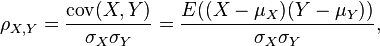
where E is the expected value operator and cov means covariance. Since μX = E(X), σX2 = E(X2) − E2(X) and likewise for Y, we may also write

\rho_{X,Y}=\frac{E(XY)-E(X)E(Y)}{\sqrt{E(X^2)-E^2(X)}~\sqrt{E(Y^2)-E^2(Y)}}.

The correlation is defined only if both of the standard deviations are finite and both of them are nonzero. It is a corollary of the Cauchy-Schwarz inequality that the correlation cannot exceed 1 in absolute value.

The correlation is 1 in the case of an increasing linear relationship, −1 in the case of a decreasing linear relationship, and some value in between in all other cases, indicating the degree of linear dependence between the variables. The closer the coefficient is to either −1 or 1, the stronger the correlation between the variables.

If the variables are independent then the correlation is 0, but the converse is not true because the correlation coefficient detects only linear dependencies between two variables. Here is an example: Suppose the random variable X is uniformly distributed on the interval from −1 to 1, and Y = X2. Then Y is completely determined by X, so that X and Y are dependent, but their correlation is zero; they are uncorrelated. However, in the special case when X and Y are jointly normal, independence is equivalent to uncorrelatedness.

A correlation between two variables is diluted in the presence of measurement error around estimates of one or both variables, in which case disattenuation provides a more accurate coefficient .


Positive linear correlations between 1000 pairs of numbers.  The data are graphed on the lower left and their correlation coefficients listed on the upper right.  Each square in the upper right corresponds to its mirror-image square in the lower left, the "mirror" being the diagonal of the whole array.  Each set of points correlates maximally with itself, as shown on the diagonal (all correlations = +1).
Positive linear correlations between 1000 pairs of numbers. The data are graphed on the lower left and their correlation coefficients listed on the upper right. Each square in the upper right corresponds to its mirror-image square in the lower left, the "mirror" being the diagonal of the whole array. Each set of points correlates maximally with itself, as shown on the diagonal (all correlations = +1).

The sample correlation

If we have a series of n measurements of X and Y written as xi and yi where i = 1, 2, ..., n, then the Pearson product-moment correlation coefficient can be used to estimate the correlation of X and Y . The Pearson coefficient is also known as the "sample correlation coefficient". It is especially important if X and Y are both normally distributed. The Pearson correlation coefficient is then the best estimate of the correlation of X and Y . The Pearson correlation coefficient is written:

r_{xy}=\frac{\sum (x_i-\bar{x})(y_i-\bar{y})}{(n-1) s_x s_y},

where \bar{x} and \bar{y} are the sample means of X and Y , sx and sy are the sample standard deviations of X and Y and the sum is from i = 1 to n. As with the population correlation, we may rewrite this as

r_{xy}=\frac{n\sum x_iy_i-\sum x_i\sum y_i} {\sqrt{n\sum x_i^2-(\sum x_i)^2}~\sqrt{n\sum y_i^2-(\sum y_i)^2}}.

Again, as is true with the population correlation, the absolute value of the sample correlation must be less than or equal to 1. Though the above formula conveniently suggests a single-pass algorithm for calculating sample correlations, it is notorious for its numerical instability (see below for something more accurate).

The square of the sample correlation coefficient, which is also known as the coefficient of determination, is the fraction of the variance in yi that is accounted for by a linear fit of xi to yi . This is written

r_{xy}^2=1-\frac{s_{y|x}^2}{s_y^2},

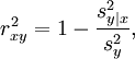
where sy|x2 is the square of the error of a linear regression of xi on yi by the equation y = a + bx:

s_{y|x}^2=\frac{1}{n-1}\sum_{i=1}^n (y_i-a-bx_i)^2,

and sy2 is just the variance of y:

s_y^2=\frac{1}{n-1}\sum_{i=1}^n (y_i-\bar{y})^2.

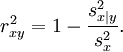
Note that since the sample correlation coefficient is symmetric in xi and yi , we will get the same value for a fit of xi to yi :

r_{xy}^2=1-\frac{s_{x|y}^2}{s_x^2}.

This equation also gives an intuitive idea of the correlation coefficient for higher dimensions. Just as the above described sample correlation coefficient is the fraction of variance accounted for by the fit of a 1-dimensional linear submanifold to a set of 2-dimensional vectors (xi , yi ), so we can define a correlation coefficient for a fit of an m-dimensional linear submanifold to a set of n-dimensional vectors. For example, if we fit a plane z = a + bx + cy to a set of data (xi , yi , zi ) then the correlation coefficient of z to x and y is

r^2=1-\frac{\sigma_{z|xy}^2}{s_z^2}.

Geometric Interpretation of correlation

The correlation coefficient can also be viewed as the cosine of the angle between the two vectors of samples drawn from the two random variables.

Caution: This method only works with centered data, i.e., data which have been shifted by the sample mean so as to have an average of zero. Some practitioners prefer an uncentered (non-Pearson-compliant) correlation coefficient. See the example below for a comparison.

As an example, suppose five countries are found to have gross national products of 1, 2, 3, 5, and 8 billion dollars, respectively. Suppose these same five countries (in the same order) are found to have 11%, 12%, 13%, 15%, and 18% poverty. Then let x and y be ordered 5-element vectors containing the above data: x = (1, 2, 3, 5, 8) and y = (0.11, 0.12, 0.13, 0.15, 0.18).

By the usual procedure for finding the angle between two vectors (see dot product), the uncentered correlation coefficient is:

 \cos \theta = \frac { \bold{x} \cdot \bold{y} } { \left\| \bold{x} \right\| \left\| \bold{y} \right\| } = \frac { 2.93 } { \sqrt { 103 } \sqrt { 0.0983 } } = 0.920814711.

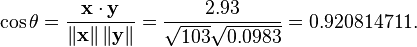
Note that the above data were deliberately chosen to be perfectly correlated: y = 0.10 + 0.01 x. The Pearson correlation coefficient must therefore be exactly one. Centering the data (shifting x by E(x) = 3.8 and y by E(y) = 0.138) yields x = (-2.8, -1.8, -0.8, 1.2, 4.2) and y = (-0.028, -0.018, -0.008, 0.012, 0.042), from which
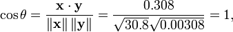
 \cos \theta = \frac { \bold{x} \cdot \bold{y} } { \left\| \bold{x} \right\| \left\| \bold{y} \right\| } = \frac { 0.308 } { \sqrt { 30.8 } \sqrt { 0.00308 } } = 1,

as expected.

Interpretation of the size of a correlation

Correlation Negative Positive
Small −0.29 to −0.10 0.10 to 0.29
Medium −0.49 to −0.30 0.30 to 0.49
Large −1.00 to −0.50 0.50 to 1.00

Several authors have offered guidelines for the interpretation of a correlation coefficient. Cohen (1988),[1] for example, has suggested the following interpretations for correlations in psychological research, in the table on the right.

As Cohen himself has observed, however, all such criteria are in some ways arbitrary and should not be observed too strictly. This is because the interpretation of a correlation coefficient depends on the context and purposes. A correlation of 0.9 may be very low if one is verifying a physical law using high-quality instruments, but may be regarded as very high in the social sciences where there may be a greater contribution from complicating factors.

Non-parametric correlation coefficients

Pearson's correlation coefficient is a parametric statistic, and it may be less useful if the underlying assumption of normality is violated. Non-parametric correlation methods, such as Chi-square, Point biserial correlation, Spearman's ρ and Kendall's τ may be useful when distributions are not normal; they are a little less powerful than parametric methods if the assumptions underlying the latter are met, but are less likely to give distorted results when the assumptions fail.

Other measures of dependence among random variables

To get a measure for more general dependencies in the data (also nonlinear) it is better to use the correlation ratio which is able to detect almost any functional dependency, or mutual information/total correlation which is capable of detecting even more general dependencies.

Copulas and correlation

The information given by a correlation coefficient is not enough to define the dependence structure between random variables; to fully capture it we must consider a copula between them. The correlation coefficient completely defines the dependence structure only in very particular cases, for example when the cumulative distribution functions are the multivariate normal distributions. In the case of elliptic distributions it characterizes the (hyper-)ellipses of equal density, however, it does not completely characterize the dependence structure (for example, the a multivariate t-distribution's degrees of freedom determine the level of tail dependence).

Correlation matrices

The correlation matrix of n random variables X1, ..., Xn is the n × n matrix whose i,j entry is corr(Xi, Xj). If the measures of correlation used are product-moment coefficients, the correlation matrix is the same as the covariance matrix of the standardized random variables Xi /SD(Xi) for i = 1, ..., n. Consequently it is necessarily a positive-semidefinite matrix.

The correlation matrix is symmetric because the correlation between Xi and Xj is the same as the correlation between Xj and Xi.

Removing correlation

It is always possible to remove the correlation between zero-mean random variables with a linear transform, even if the relationship between the variables is nonlinear. Suppose a vector of n random variables is sampled m times. Let X be a matrix where Xi,j is the jth variable of sample i. Let Zr,c be an r by c matrix with every element 1. Then D is the data transformed so every random variable has zero mean, and T is the data transformed so all variables have zero mean, unit variance, and zero correlation with all other variables.

D = X -\frac{1}{m} Z_{m,m} X
T = D (D^T D)^{-\frac{1}{2}}

where an exponent of -1/2 represents the matrix square root of the inverse of a matrix. The covariance matrix of T will be the identity matrix. If a new data sample x is a row vector of n elements, then the same transform can be applied to x to get the transformed vectors d and t:

d = x - \frac{1}{m} Z_{1,m} X
t = d (D^T D)^{-\frac{1}{2}}.

Common misconceptions about correlation

Correlation and causality

The conventional dictum that "correlation does not imply causation" means that correlation cannot be validly used to infer a causal relationship between the variables. This dictum should not be taken to mean that correlations cannot indicate causal relations. However, the causes underlying the correlation, if any, may be indirect and unknown. Consequently, establishing a correlation between two variables is a not sufficient condition to establish a causal relationship (in either direction).

Here is a simple example: hot weather may cause both crime and ice-cream purchases. Therefore crime is correlated with ice-cream purchases. But crime does not cause ice-cream purchases and ice-cream purchases do not cause crime.

A correlation between age and height in children is fairly causally transparent, but a correlation between mood and health in people is less so. Does improved mood lead to improved health? Or does good health lead to good mood? Or does some other factor underlie both? Or is it pure coincidence? In other words, a correlation can be taken as evidence for a possible causal relationship, but cannot indicate what the causal relationship, if any, might be.

Correlation and linearity

Four sets of data with the same correlation of 0.81

While Pearson correlation indicates the strength of a linear relationship between two variables, its value alone may not be sufficient to evaluate this relationship, especially in the case where the assumption of normality is incorrect.

The image on the right shows scatterplots of Anscombe's quartet, a set of four different pairs of variables created by Francis Anscombe.[2] The four y variables have the same mean (7.5), standard deviation (4.12), correlation (0.81) and regression line (y = 3 + 0.5x). However, as can be seen on the plots, the distribution of the variables is very different. The first one (top left) seems to be distributed normally, and corresponds to what one would expect when considering two variables correlated and following the assumption of normality. The second one (top right) is not distributed normally; while an obvious relationship between the two variables can be observed, it is not linear, and the Pearson correlation coefficient is not relevant. In the third case (bottom left), the linear relationship is perfect, except for one outlier which exerts enough influence to lower the correlation coefficient from 1 to 0.81. Finally, the fourth example (bottom right) shows another example when one outlier is enough to produce a high correlation coefficient, even though the relationship between the two variables is not linear.

These examples indicate that the correlation coefficient, as a summary statistic, cannot replace the individual examination of the data.

Computing correlation accurately in a single pass

The following algorithm (in pseudocode) will estimate correlation with good numerical stability

sum_sq_x = 0
sum_sq_y = 0
sum_coproduct = 0
mean_x = x[1]
mean_y = y[1]
for i in 2 to N:
sweep = (i - 1.0) / i
delta_x = x[i] - mean_x
delta_y = y[i] - mean_y
sum_sq_x += delta_x * delta_x * sweep
sum_sq_y += delta_y * delta_y * sweep
sum_coproduct += delta_x * delta_y * sweep
mean_x += delta_x / i
mean_y += delta_y / i
pop_sd_x = sqrt( sum_sq_x / N )
pop_sd_y = sqrt( sum_sq_y / N )
cov_x_y = sum_coproduct / N
correlation = cov_x_y / (pop_sd_x * pop_sd_y)

For an enlightening experiment, check the correlation of {900,000,000 + i for i=1...100} with {900,000,000 - i for i=1...100}, perhaps with a few values modified. Poor algorithms will fail.

Currency correlation

Currency correlation is correlation between two currency pairs, or more generally, correlations between values of commodities, stocks and bonds markets. It is used as a tool to predict changes in market value.