analysis of variance ANOVA

One-way analysis of variance

Note:

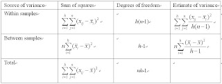
(1) The within-samples estimate does not depend on the mean for any individual: had, for example, all of the ith sample’s measurements been increased by say, 5, this estimate of the variance would be unaltered. However, had the variability of the ith sample’s measurements increased, so would this estimate of that variance.

(2) The between-samples estimate does not depend on the ‘within-sample’ variability because it is calculated using the means of the samples. However, if one of these means is altered so is the estimate of variance. In particular, as the difference between the means increases so does the ‘between-class’ estimate of variance.

(3) To test whether the variances is significantly different from each other, we use the F-test.

Two-way analysis of variance

Example see http://www.mnstate.edu/wasson/ed602lesson13.htm

Example problem using One-way Analysis of Variance

Three groups of students, 5 in each group, were receiving therapy for severe test anxiety. Group 1 received 5 hours of therapy, group 2 - 10 hours and group 3 - 15 hours. At the end of therapy each subject completed an evaluation of test anxiety (the dependent variable in the study). Did the amount of therapy have an effect on the level of test anxiety?

The three groups of students received the following scores on the Test Anxiety Index (TAI) at the end of treatment.

TAI Scores for Three Groups of Students

Group 1 - 5 hours	Group 2 - 10 hours	Group 3 - 15 hours
48	55	51
50	52	52
53	53	50
52	55	53
50	53	50

The following table contains the quantities we need to calculate the means for the three groups, the sum of squares, and the degrees of freedom:

Worksheet for Test Anxiety Study

Group 1 - 5 hours		Group 2 - 10 hours		Group 3 - 15 hours
X1	(X1)2	X2	(X2)2	X3	(X3)2
48	2304	55	3025	51	2601
50	2500	52	2704	52	2704
53	2809	53	2809	50	2500
52	2704	55	3025	53	2809
50	2500	53	2809	50	2500
----------	----------	----------	----------	----------	----------
253	12817	268	14372	256	13114

The mean for group 1 is 253/5 = 50.6, the mean for group 2 is 268/5 = 53.6, and the mean for group 3 is 256/5 = 51.2

Is the differences between these three means significant? We can use analysis of variance to answer that question. Since we only have one independent variable, amount of therapy, we will use one-way analysis of variance. If we were concerned with the effect of two independent variables on the dependent variable, then we would use two-way analysis of variance.

First we will calculate SS_B, the sum of squares between groups, where X₁ is a score from Group 1, X₂ is a score from Group 2, X₃ is a score from Group 3, n₁ is the number of subjects in group 1, n₂ is the number of subjects in group 2, n₃ is the number of subjects in group 3, X_T is a score from any subject in the total group of subjects, and N_T is the total number of subjects in all groups.

The degrees of freedom between groups is:

df_B = K - 1 = 3 - 1 = 2

Where K is the number of groups.

Next we calculate SS_W, the sum of squares within groups.

The degrees of freedom within groups is:

df_W = N_T - K = 15 - 3 = 12

Where N_T is the total number of subjects.

Finally, we will calculate SS_T, the total sum of squares.

As a check SS_T = SS_B + SS_W

54.4 = 25.2 + 29.2

We can now calculate MS_B, the mean square between groups, MS_W, the mean square within groups, and F, the F ratio.

To test the significance of the F value we obtained, we need to compare it with the critical F value with an alpha level of .05, 2 degrees of freedom between groups (or degrees of freedom in the numerator of the F ratio), and 12 degrees of freedom within groups (or degrees of freedom in the denominator of the F ratio). We can look up the critical value of F in Appendix Table D of the text book (The 5 percent (Lightface Type) and 1 percent (Boldface Type) points for the Distribution of F), pages 319-326. Look in the table under column 2 (2 degrees of freedom for the numerator) and row 12 (12 degrees of freedom for the denominator) and read the non-boldfaced entry (for .05 level) of 3.88 - this is the critical value for F.

One way of indicating this critical value of F at the .05 level, with 2 degrees of freedom between groups and 12 degrees of freedom within groups is

F_.05(2,12) = 3.88

When using analysis of variance, it is a common practice to present the results of the analysis in an analysis of variance table. This table which shows the source of variation, the sum of squares, the degrees of freedom, the mean squares, and the probability is sometimes presented in a research article. The analysis of variance table for our problem would appear as follows:

Analysis of Variance Table

Source of Variation	Sum of Squares	Degrees of Freedom	Mean Square	F Ratio	p
Between Groups	25.20	2	12.60	5.178	<.05
Within Groups	29.20	12	2.43
Total	54.40	14