Definitions
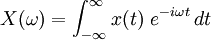
There are several common conventions for defining the Fourier transform of a complex-valued Lebesgue integrable function,  In communications and signal processing, for instance, it is often the function:
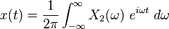
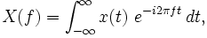 for every real number
When the independent variable  represents time (with SI unit of seconds), the transform variable
  represents ordinary frequency (in hertz). The complex-valued function,
  is said to represent
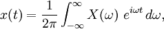
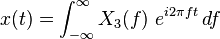
  in the frequency domain. I.e., if is a continuous function, then it can be reconstructed from
  by the inverse transform:
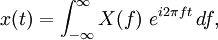 for every real number
Other notations for  are:
are:  and
and 
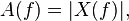
The interpretation of is aided by expressing it in polar coordinate form: 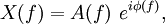 where:
 the
the  the
the Then the inverse transform can be written:

which is a recombination of all the frequency components of  Each component is a complex sinusoid of the form ei2πft whose amplitude is A(f) and whose initial phase angle (at t = 0) is φ(f).
In mathematics, the Fourier transform is commonly written in terms of angular frequency:  whose units are radians per second.
The substitution  into the formulas above produces this convention:
which is also a bilateral Laplace transform evaluated at s = iω.However, this destroys the symmetry, resulting in the transform pair
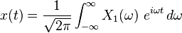
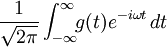
To restore the symmetry of the transforms, the 2π factor can be split evenly between the Fourier transform and the inverse, which leads to another popular convention:
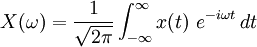

This convention and the X(f) convention are unitary transforms.
Variations of all three conventions can be created by conjugating the complex-exponen
| angular frequency  (rad/s) | unitary | 
|
| non-unitary | 
| |
| ordinary frequency (hertz) | unitary | 
|
Generalization
There are several ways to define the Fourier transform pair. The "forward" and "inverse" transforms are always defined so that the operation of both transforms in either order on a function will return the original function. In other words, the composition of the transform pair is defined to be the identity transformation. Using two arbitrary real constants a and b, the most general definition of the forward 1-dimensional Fourier transform is given by

and the inverse is given by

Note that the transform definitions are symmetric; they can be reversed by simply changing the signs of a and b.
The convention adopted in this article is (a,b) = (0,1). The choice of a and b is usually chosen so that it is geared towards the context in which the transform pairs are being used. The non-unitary convention above is (a,b) = (1,1). Another very common definition is (a,b) = (0,2π) which is often used in signal processing applications. In this case, the angular frequency ω becomes ordinary frequency f. If f (or ω) and t carry units, then their product must be dimensionless. For example, t may be in units of time, specifically seconds, and f (or ω) would be in hertz (or radian/s).
The Fourier transform  of a function
  is implemented as FourierTransfor
 and
and  can be used by passing the optional FourierParamete
 a, b
a, b option. By default, Mathematica takes FourierParamete
 . Unfortunately, a number of other conventions are in widespread use. For example,
  is used in modern physics,
  is used in pure mathematics and systems engineering,
  is used in probability theory for the computation of the characteristic function,
  is used in classical physics, and
  is used in signal processing. In this work, following Bracewell (1999, pp. 6-7), it is always assumed that
  and
and  unless otherwise stated. This choice often results in greatly simplified transforms of common functions such as 1,
  , etc.
Since any function can be split up into even and odd portions  and
and  ,
,
| (11) |
a Fourier transform can always be expressed in terms of the Fourier cosine transform and Fourier sine transform as
Table of important Fourier transforms
The following table records some important Fourier transforms. G and H denote Fourier transforms of g(t) and h(t), respectively. g and h may be integrable functions or tempered distributions. Note that the two most common unitary conventions are included.
Functional relationships
| Signal | Fourier transform unitary, angular frequency | Fourier transform unitary, ordinary frequency | Remarks | |
|---|---|---|---|---|
 |   |   | ||
| 101 |  | 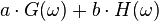 | 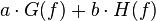 | Linearity |
| 102 |  |  |  | Shift in time domain |
| 103 |  |  |  | Shift in frequency domain, dual of 2 |
| 104 |  |  |  | If  is large, then is concentrated around 0 and spreads out and flattens. It is interesting to consider the limit of this as | a | tends to infinity - the delta function is large, then is concentrated around 0 and spreads out and flattens. It is interesting to consider the limit of this as | a | tends to infinity - the delta function |
| 105 |  |  |  | Duality property of the Fourier transform. Results from swapping "dummy" variables of and . |
| 106 |  |  |  | Generalized derivative property of the Fourier transform |
| 107 |  |  | 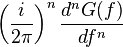 | This is the dual of 106 |
| 108 |  |  |  |  denotes the convolution of denotes the convolution of  and and  — this rule is the convolution theorem — this rule is the convolution theorem |
| 109 |  |  |  | This is the dual of 108 |
| 110 | is purely real, and an even function |  and and  are purely real, and even functions are purely real, and even functions | ||
| 111 | is purely real, and an odd function | and are purely imaginary, and odd functions | ||
Square-integrable functions
| Signal | Fourier transform unitary, angular frequency | Fourier transform unitary, ordinary frequency | Remarks | |
|---|---|---|---|---|
|   |   | ||
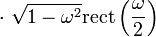
| 201 |  |  |  | The rectangular pulse and the normalized sinc function |
| 202 |  |  | 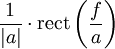 | Dual of rule 201. The rectangular function is an idealized low-pass filter, and the sinc function is the non-causal impulse response of such a filter. |
| 203 |  |  | 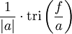 | tri is the triangular function |
| 204 |  | 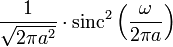 | 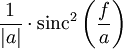 | Dual of rule 203. |
| 205 |  |  |  | Shows that the Gaussian function exp( − αt2) is its own Fourier transform. For this to be integrable we must have |
| 206 | 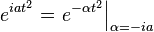 | 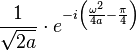 | 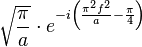 | common in optics |
| 207 |  |  | 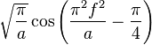 | |
| 208 |  |  |  | |
| 209 |  |  |  | a>0 |
| 210 |  |  |  | the transform is the function itself |
| 211 |  |  |  | J0(t) is the Bessel function of first kind of order 0 |
| 212 |  | 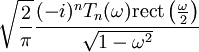 |  | it's the generalization of the previous transform; Tn (t) is the Chebyshev polynomial of the first kind. |
| 213 |  | 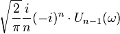 | 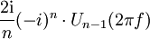 | Un (t) is the Chebyshev polynomial of the second kind |
| 214 |  | 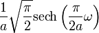 |  | Hyperbolic secant is its own Fourier transform |

Distributions
| Signal | Fourier transform unitary, angular frequency | Fourier transform unitary, ordinary frequency | Remarks | |
|---|---|---|---|---|
| | | ||
| 301 |  |  |  |  denotes the Dirac delta distribution. denotes the Dirac delta distribution. |
| 302 |  |  | | Dual of rule 301. |
| 303 |  | 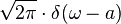 |  | This follows from and 103 and 302. |
| 304 |  | 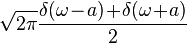 | 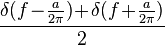 | Follows from rules 101 and 303 using Euler's formula:  |
| 305 |  | 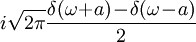 |  | Also from 101 and 303 using  |
| 306 |  |  |  | Here,  is a natural number. is a natural number.  is the -th distribution derivative of the Dirac delta. This rule follows from rules 107 and 302. Combining this rule with 1, we can transform all polynomials. is the -th distribution derivative of the Dirac delta. This rule follows from rules 107 and 302. Combining this rule with 1, we can transform all polynomials. |
| 307 |  | 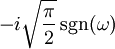 |  | Here  is the sign function; note that this is consistent with rules 107 and 302. is the sign function; note that this is consistent with rules 107 and 302. |
| 308 |  |  |  | Generalization of rule 307. |
| 309 |  |  |  | The dual of rule 307. |
| 310 |  | 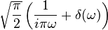 |  | Here u(t) is the Heaviside unit step function; this follows from rules 101 and 309. |
| 311 |  | 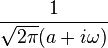 |  | u(t) is the Heaviside unit step function and a > 0. |
| 312 |  |  | 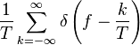 | The Dirac comb — helpful for explaining or understanding the transition from continuous to discrete time. |
Fourier transform properties
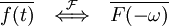
Notation:  denotes that f(t) and F(ω) are a Fourier transform pair.
- Linearity
-
-

- Convolution
-
-

- Conjugation
-
-
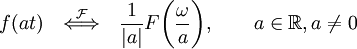
- Scaling
-
-
- Time reversal
-
-

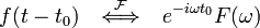
- Time shift
-
-
- Modulation (multiplication
by complex exponential) -
-

- Multiplication by sin ω0t
-
-
![f(t)\sin \omega_{0}t \quad \stackrel{\mathcal{F}}{\Longleftrightarrow}\quad \frac{i}{2}[F(\omega+\omega_{0})-F(\omega-\omega_{0})]\,](http://upload.wikimedia.org/math/2/6/c/26c02062665c7123a30cbddc1155da70.png)
- Multiplication by cos ω0t
-
-
![f(t)\cos \omega_{0}t \quad \stackrel{\mathcal{F}}{\Longleftrightarrow}\quad \frac{1}{2}[F(\omega+\omega_{0})+F(\omega-\omega_{0})]\,](http://upload.wikimedia.org/math/b/8/e/b8e63221e47e710aa1e28abb415c4cb5.png)
- Integration
-
-

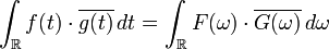
- Parseval's theorem
-
-

No comments:
Post a Comment