
Showing posts with label Data Mining: Graph. Show all posts
Showing posts with label Data Mining: Graph. Show all posts
Wednesday, 28 November 2007


Friday, 19 October 2007
Confusion Matrix
A confusion matrix (Kohavi and Provost, 1998) contains information about actual and predicted classifications done by a classification system. Performance of such systems is commonly evaluated using the data in the matrix. The following table shows the confusion matrix for a two class classifier.
 [1]
 [2]
 [3]
 [4]
 [5]
 [6]
The entries in the confusion matrix have the following meaning in the context of our study:
- a is the number of correct predictions that an instance is negative,
- b is the number of incorrect predictions that an instance is positive,
- c is the number of incorrect of predictions that an instance negative, and
- d is the number of correct predictions that an instance is positive.
| Predicted | |||
| Negative | Positive | ||
| Actual | Negative | a | b |
Several standard terms have been defined for the 2 class matrix:
- The accuracy (AC) is the proportion of the total number of predictions that were correct. It is determined using the equation:
[1]- The recall or hit rate or true positive rate (TP) is the proportion of positive cases that were correctly identified, as calculated using the equation:
[2]- The false alarm rate or false positive rate (FP) is the proportion of negatives cases that were incorrectly classified as positive, as calculated using the equation:
[3]- The true negative rate (TN) is defined as the proportion of negatives cases that were classified correctly, as calculated using the equation:
[4]- The false negative rate (FN) is the proportion of positives cases that were incorrectly classified as negative, as calculated using the equation:
[5]- Finally, precision (P) is the proportion of the predicted positive cases that were correct, as calculated using the equation:
[6]The accuracy determined using equation 1 may not be an adequate performance measure when the number of negative cases is much greater than the number of positive cases (Kubat et al., 1998). Suppose there are 1000 cases, 995 of which are negative cases and 5 of which are positive cases. If the system classifies them all as negative, the accuracy would be 99.5%, even though the classifier missed all positive cases. Other performance measures account for this by including TP in a product: for example, geometric mean (g-mean) (Kubat et al., 1998), as defined in equations 7 and 8, and F-Measure (Lewis and Gale, 1994), as defined in equation 9.
 [7]
 [8]
 [9]
In equation 9, b has a value from 0 to infinity and is used to control the weight assigned to TP and P. Any classifier evaluated using equations 7, 8 or 9 will have a measure value of 0, if all positive cases are classified incorrectly.
Another way to examine the performance of classifiers is to use a ROC graph, described on the next page.
ROC Graph
ROC graphs are another way besides confusion matrices to examine the performance of classifiers (Swets, 1988). A ROC graph is a plot with the false positive rate on the X axis and the true positive rate on the Y axis. The point (0,1) is the perfect classifier: it classifies all positive cases and negative cases correctly. It is (0,1) because the false positive rate is 0 (none), and the true positive rate is 1 (all). The point (0,0) represents a classifier that predicts all cases to be negative, while the point (1,1) corresponds to a classifier that predicts every case to be positive. Point (1,0) is the classifier that is incorrect for all classifications. In many cases, a classifier has a parameter that can be adjusted to increase TP at the cost of an increased FP or decrease FP at the cost of a decrease in TP. Each parameter setting provides a (FP, TP) pair and a series of such pairs can be used to plot an ROC curve. A non-parametric classifier is represented by a single ROC point, corresponding to its (FP,TP) pair.
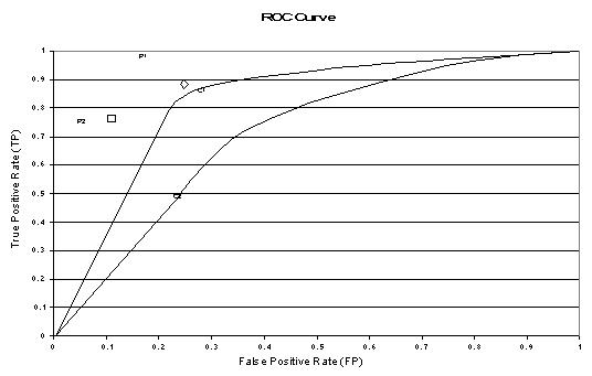
The above figure shows an example of an ROC graph with two ROC curves labeled C1 and C2, and two ROC points labeled P1 and P2. Non-parametric algorithms produce a single ROC point for a particular data set.
Features of ROC Graphs
- An ROC curve or point is independent of class distribution or error costs (Provost et al., 1998).
- An ROC graph encapsulates all information contained in the confusion matrix, since FN is the complement of TP and TN is the complement of FP (Swets, 1988).
- ROC curves provide a visual tool for examining the tradeoff between the ability of a classifier to correctly identify positive cases and the number of negative cases that are incorrectly classified.
- The closer the curve follows the left-hand border and then the top border of the ROC space, the more accurate the test.The closer the curve comes to the 45-degree diagonal of the ROC space, the less accurate the test.
Area-based Accuracy Measure
It has been suggested that the area beneath an ROC curve can be used as a measure of accuracy in many applications (Swets, 1988). Provost and Fawcett (1997) argue that using classification accuracy to compare classifiers is not adequate unless cost and class distributions are completely unknown and a single classifier must be chosen to handle any situation. They propose a method of evaluating classifiers using a ROC graph and imprecise cost and class distribution information.
Euclidian Distance Comparison
Another way of comparing ROC points is by using an equation that equates accuracy with the Euclidian distance from the perfect classifier, point (0,1) on the graph. We include a weight factor that allows us to define relative misclassification costs, if such information is available. We define ACd as a distance based performance measure for an ROC point and calculate it using the equation:
 [22]
where W is a factor, ranging from 0 to 1, that is used to assign relative importance to false positives and false negatives. ACd ranges from 0 for the perfect classifier to sqrt(2) for a classifier that classifies all cases incorrectly, point (1,0) on the ROC graph. ACd differs from g-mean1, g-mean2 and F-measure in that it is equal to zero only if all cases are classified correctly. In other words, a classifier evaluated using ACd gets some credit for correct classification of negative cases, regardless of its accuracy in correctly identifying positive cases.
Example
Consider two algorithms A and B that perform adequately against most data sets. However, assume both A and B misclassify all positive cases in a particular data set and A classifies 10 times the number of infrequent itemsets as potentially frequent compared to B. Algorithm B is the better algorithm in this case because there has been less wasted effort counting infrequent itemsets.
Cumulative Gains and Lift Charts
- Lift is a measure of the effectiveness of a predictive model calculated as the ratio between the results obtained with and without the predictive model.
- Cumulative gains and lift charts are visual aids for measuring model performance
- Both charts consist of a lift curve and a baseline
- The greater the area between the lift curve and the baseline, the better the model
Example Problem 1
A company wants to do a mail marketing campaign. It costs the company $1 for each item mailed. They have information on 100,000 customers. Create a cumulative gains and a lift chart from the following data.- Overall Response Rate: If we assume we have no model other than the prediction of the overall response rate, then we can predict the number of positive responses as a fraction of the total customers contacted. Suppose the response rate is 20%. If all 100,000 customers are contacted we will receive around 20,000 positive responses.
| Cost ($) | Total Customers Contacted | Positive Responses |
|---|---|---|
| 100000 | 100000 | 20000 |
- Prediction of Response Model: A response model predicts who will respond to a marketing campaign. If we have a response model, we can make more detailed predictions. For example, we use the response model to assign a score to all 100,000 customers and predict the results of contacting only the top 10,000 customers, the top 20,000 customers, etc.
| Cost ($) | Total Customers Contacted | Positive Responses |
|---|---|---|
| 10000 | 10000 | 6000 |
| 20000 | 20000 | 10000 |
| 30000 | 30000 | 13000 |
| 40000 | 40000 | 15800 |
| 50000 | 50000 | 17000 |
| 60000 | 60000 | 18000 |
| 70000 | 70000 | 18800 |
| 80000 | 80000 | 19400 |
| 90000 | 90000 | 19800 |
| 100000 | 100000 | 20000 |
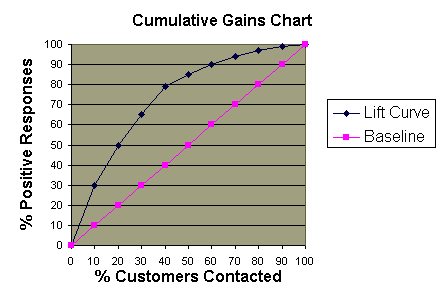
Cumulative Gains Chart:
- The y-axis shows the percentage of positive responses. This is a percentage of the total possible positive responses (20,000 as the overall response rate shows).
- The x-axis shows the percentage of customers contacted, which is a fraction of the 100,000 total customers.
- Baseline (overall response rate): If we contact X% of customers then we will receive X% of the total positive responses.
- Lift Curve: Using the predictions of the response model, calculate the percentage of positive responses for the percent of customers contacted and map these points to create the lift curve.
Lift Chart:
- Shows the actual lift.
- To plot the chart: Calculate the points on the lift curve by determining the ratio between the result predicted by our model and the result using no model.
- Example: For contacting 10% of customers, using no model we should get 10% of responders and using the given model we should get 30% of responders. The y-value of the lift curve at 10% is 30 / 10 = 3.
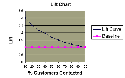
Analyzing the Charts: Cumulative gains and lift charts are a graphical representation of the advantage of using a predictive model to choose which customers to contact. The lift chart shows how much more likely we are to receive respondents than if we contact a random sample of customers. For example, by contacting only 10% of customers based on the predictive model we will reach 3 times as many respondents as if we use no model.
Evaluating a Predictive Model
We can assess the value of a predictive model by using the model to score a set of customers and then contacting them in this order. The actual response rates are recorded for each cutoff point, such as the first 10% contacted, the first 20% contacted, etc. We create cumulative gains and lift charts using the actual response rates to see how much the predictive model would have helped in this situation. The information can be used to determine whether we should use this model or one similar to it in the future.Example Problem 2
Using the response model P(x)=100-AGE(x) for customer x and the data table shown below, construct the cumulative gains and lift charts. Ties in ranking should be arbitrarily broken by assigning a higher rank to who appears first in the table.| | | | |
| | | | |
| | | | |
| | | | |
| | | | |
| | | | |
| | | | |
| | | | |
| | | | |
| | | | |
| | | | |
| | | | |
| | | | |
| | | | |
| | | | |
| | | | |
| | | | |
| | | | |
| | | | |
| | | | |
| | | | |
1. Calculate P(x) for each person x
2. Order the people according to rank P(x)
3. Calculate the percentage of total responses for each cutoff point
Customer Name P(x) Actual Response Alex 88 Y Amy 87 N Hilary 81 Y Philip 80 Y Bob 79 Y Catherine 77 N Nancy 76 Y Jessica 75 Y Preston 75 N Laura 71 Y Elizabeth 70 Y Kim 69 N Erin 65 Y Alan 61 N Chris 58 N Fred 52 N Margot 49 N Trent 45 N Sean 35 Y John 24 N
- Response Rate = Number of Responses / Total Number of Responses (10)
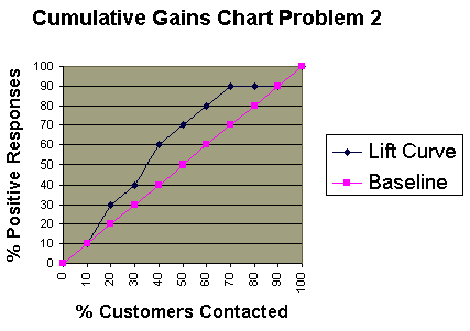
4. Create the cumulative gains chart:
Total Customers Contacted Number of Responses Response Rate
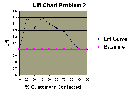
- The lift curve and the baseline have the same values for 10%-20% and 90%-100%.
5. Create the lift chart:
Introduction to ROC Curves
A ROC curve provides a graphical representation of the relationship between the true-positive and false-positive prediction rate of a model. The y-axis corresponds to the sensitivity of the model, i.e. how well the model is able to predict true positives (real cleavages) from sites that are not cleaved, and the y-coordinates are calculated as:

The x-axis corresponds to the specificity (expressed on the curve as 1-specificity), i.e. the ability of the model to identify true negatives. An increase in specificity (i.e. a decrease along the X-axis) results in an increase in sensitivity. The x-coordinates are calculated as:

The greater the sensitivity at high specificity values (i.e. high y-axis values at low X-axis values) the better the model. A numerical measure of the accuracy of the model can be obtained from the area under the curve, where an area of 1.0 signifies near perfect accuracy, while an area of less than 0.5 indicates that the model is worse than just random. The quantitative-qualitative relationship between area and accuracy follows a fairly linear pattern, such that the following could be used as a guide:
- 0.9-1: Excellent
- 0.8-0.9: Very good
- 0.7-0.8: Good
- 0.6-0.7: Average
- 0.5-0.6: Poor
Introduction to ROC Curves
 The sensitivity and specificity of a diagnostic test depends on more than just the "quality" of the test--they also depend on the definition of what constitutes an abnormal test. Look at the the idealized graph at right showing the number of patients with and without a disease arranged according to the value of a diagnostic test. This distributions overlap--the test (like most) does not distinguish normal from disease with 100% accuracy. The area of overlap indicates where the test cannot distinguish normal from disease. In practice, we choose a cutpoint (indicated by the vertical black line) above which we consider the test to be abnormal and below which we consider the test to be normal. The position of the cutpoint will determine the number of true positive, true negatives, false positives and false negatives. We may wish to use different cutpoints for different clinical situations if we wish to minimize one of the erroneous types of test results.
We can use the hypothyroidism data from the likelihood ratio section to illustrate how sensitivity and specificity change depending on the choice of T4 level that defines hypothyroidism. Recall the data on patients with suspected hypothyroidism reported by Goldstein and Mushlin (J Gen Intern Med 1987;2:20-24.). The data on T4 values in hypothyroid and euthyroid patients are shown graphically (below left) and in a simplified tabular form (below right). 
| T4 value | Hypothyroid | Euthyroid |
| 5 or less | 18 | 1 |
| 5.1 - 7 | 7 | 17 |
| 7.1 - 9 | 4 | 36 |
| 9 or more | 3 | 39 |
| Totals: | 32 | 93 |
Suppose that patients with T4 values of 5 or less are considered to be hypothyroid. The data display then reduces to:
| T4 value | Hypothyroid | Euthyroid |
| 5 or less | 18 | 1 |
| > 5 | 14 | 92 |
| Totals: | 32 | 93 |
Now, suppose we decide to make the definition of hypothyroidism less stringent and now consider patients with T4 values of 7 or less to be hypothyroid. The data display will now look like this:
| T4 value | Hypothyroid | Euthyroid |
| 7 or less | 25 | 18 |
| > 7 | 7 | 75 |
| Totals: | 32 | 93 |
Lets move the cut point for hypothyroidism one more time:
| T4 value | Hypothyroid | Euthyroid |
| <> | 29 | 54 |
| 9 or more | 3 | 39 |
| Totals: | 32 | 93 |
Now, take the sensitivity and specificity values above and put them into a table:
| Cutpoint | Sensitivity | Specificity |
| 5 | 0.56 | 0.99 |
| 7 | 0.78 | 0.81 |
| 9 | 0.91 | 0.42 |
The next section covers how to use the numbers we just calculated to draw and interpret an ROC curve.
.
|
Plotting and Intrepretating an ROC Curve
| T4 value | Hypothyroid | Euthyroid |
| 5 or less | 18 | 1 |
| 5.1 - 7 | 7 | 17 |
| 7.1 - 9 | 4 | 36 |
| 9 or more | 3 | 39 |
| Totals: | 32 | 93 |
| Cutpoint | Sensitivity | Specificity |
| 5 | 0.56 | 0.99 |
| 7 | 0.78 | 0.81 |
| 9 | 0.91 | 0.42 |
The operating characteristics (above right) can be reformulated slightly and then presented graphically as shown below to the right:
| Cutpoint | True Positives | False Positives |
| 5 | 0.56 | 0.01 |
| 7 | 0.78 | 0.19 |
| 9 | 0.91 | 0.58 |

This type of graph is called a Receiver Operating Characteristic curve (or ROC curve.) It is a plot of the true positive rate against the false positive rate for the different possible cutpoints of a diagnostic test.
An ROC curve demonstrates several things:
- It shows the tradeoff between sensitivity and specificity (any increase in sensitivity will be accompanied by a decrease in specificity).
- The closer the curve follows the left-hand border and then the top border of the ROC space, the more accurate the test.
- The closer the curve comes to the 45-degree diagonal of the ROC space, the less accurate the test.
- The slope of the tangent line at a cutpoint gives the likelihood ratio (LR) for that value of the test. You can check this out on the graph above. Recall that the LR for T4 <> 9 is 0.2. This corresponds to the far right, nearly horizontal portion of the curve.
- The area under the curve is a measure of text accuracy. This is discussed further in the next section.
.
The Area Under an ROC Curve
 The graph at right shows three ROC curves representing excellent, good, and worthless tests plotted on the same graph. The accuracy of the test depends on how well the test separates the group being tested into those with and without the disease in question. Accuracy is measured by the area under the ROC curve. An area of 1 represents a perfect test; an area of .5 represents a worthless test. A rough guide for classifying the accuracy of a diagnostic test is the traditional academic point system:
- .90-1 = excellent (A)
- .80-.90 = good (B)
- .70-.80 = fair (C)
- .60-.70 = poor (D)
- .50-.60 = fail (F)
 ROC curves can also be constructed from clinical prediction rules. The graphs at right come from a study of how clinical findings predict strep throat (Wigton RS, Connor JL, Centor RM. Transportability of a decision rule for the diagnosis of streptococcal pharyngitis. Arch Intern Med. 1986;146:81-83.) In that study, the presence of tonsillar exudate, fever, adenopathy and the absence of cough all predicted strep. The curves were constructed by computing the sensitivity and specificity of increasing numbers of clinical findings (from 0 to 4) in predicting strep. The study compared patients in Virginia and Nebraska and found that the rule performed more accurately in Virginia (area under the curve = .78) compared to Nebraska (area under the curve = .73). These differences turn out not to be statistically different, however.
At this point, you may be wondering what this area number really means and how it is computed. The area measures discrimination, that is, the ability of the test to correctly classify those with and without the disease. Consider the situation in which patients are already correctly classified into two groups. You randomly pick on from the disease group and one from the no-disease group and do the test on both. The patient with the more abnormal test result should be the one from the disease group. The area under the curve is the percentage of randomly drawn pairs for which this is true (that is, the test correctly classifies the two patients in the random pair).
Computing the area is more difficult to explain and beyond the scope of this introductory material. Two methods are commonly used: a non-parametric method based on constructing trapeziods under the curve as an approximation of area and a parametric method using a maximum likelihood estimator to fit a smooth curve to the data points. Both methods are available as computer programs and give an estimate of area and standard error that can be used to compare different tests or the same test in different patient populations. For more on quantitative ROC analysis, see Metz CE. Basic principles of ROC analysis. Sem Nuc Med. 1978;8:283-298.
A final note of historical interestYou may be wondering where the name "Reciever Operating Characteristic" came from. ROC analysis is part of a field called "Signal Dectection Therory" developed during World War II for the analysis of radar images. Radar operators had to decide whether a blip on the screen represented an enemy target, a friendly ship, or just noise. Signal detection theory measures the ability of radar receiver operators to make these important distinctions. Their ability to do so was called the Receiver Operating Characteristics. It was not until the 1970's that signal detection theory was recognized as useful for interpreting medical test results.
Subscribe to:
Posts (Atom)

